Lookup Last Value in Column or Row – Excel

This tutorial will teach you how to look up the last value in column or row in Excel.

Last Value in Column

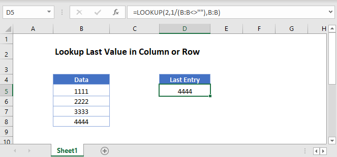
You can use the LOOKUP Function to find the last non-empty cell in a column.

=LOOKUP(2,1/(B:B<>""),B:B)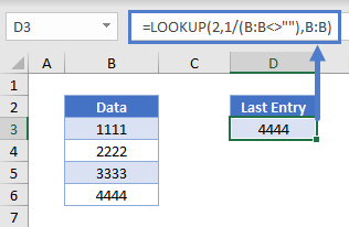

Let’s walk through this formula.

The part of the formula B:B<>”” returns an array containing True and False values: {FALSE, TRUE, TRUE,…}, testing each cell in column B is blank (FALSE).

=LOOKUP(2,1/({FALSE;TRUE;TRUE;TRUE;TRUE;TRUE;FALSE;...),B:B)

These Boolean values convert to 0 or 1 and are used to divide 1.

=LOOKUP(2,{#DIV/0!;1;1;1;1;1;#DIV/0!;,B:B)

This is the lookup_vector for the LOOKUP Function. In our case, the lookup_value is 2, but the largest value in the lookup_vector is 1, so the LOOKUP Function will match the last 1 in the array and return the corresponding value in the result_vector.

If you are sure that you only have numeric values in your column, your data start from row 1 and your data range in continuous, you can use a slightly simpler formula with the INDEX and COUNT functions.

=INDEX(B:B,COUNT(B:B))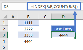

The COUNT Function returns the number of cells filled with data in the continuous range (4) and the INDEX Function thus gives the value of the cell in this corresponding row (4th).

To avoid possible errors when your range of data contains a mixture of numeric and non-numeric values, or even some blank cells, you can use the LOOKUP Function together with the ISBLANK and NOT functions.

=LOOKUP(2,1/(NOT(ISBLANK(B:B))),B:B)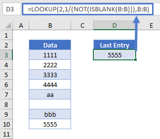

The ISBLANK Function returns an array containing True and False values, corresponding to 1’s and 0’s. The NOT Function changes True (i.e. 1) to False and False (i.e. 0) to True. If we invert this resulting array (when dividing 1 by this array), we get a result array containing again #DIV/0! errors and 1’s, which can be used as lookup array (lookup_vector) in our LOOKUP Function. The functionality of the LOOKUP Function is then the same as it was in our first example: it returns the value of the result vector at the position of the last 1 in the lookup array.

When you need the row number with the last entry to be returned, you can modify the formula used in our first example together with the ROW Function in your result_vector.

=LOOKUP(2,1/(B:B<>""),ROW(B:B))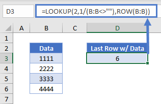

Last Value in Row

To get the last non-empty cell’s value in a row filled with numeric data, you may want to use a similar approach but with different functions: the OFFSET Function together with the MATCH and MAX functions.

=OFFSET(Reference, Rows, Columns)

=OFFSET(B2,0,MATCH(MAX(B2:XFD2)+1,B2:XFD2,1)-1)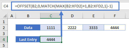

Let’s see how this formula works.

MATCH Function

We use the MATCH Function to “count” how many cell values are under 1 + the maximum of all values in row2 starting from B2.

=MATCH(lookup_value, lookup_array, [match_type])

=MATCH(MAX(B2:XFD2)+1,B2:XFD2,1)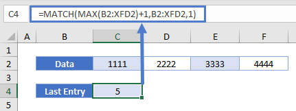

The lookup_value of the MATCH Function is the maximum of all values in the row2 + 1. Since this value obviously does not exist in the row2 and the match_type is set to 1 (less than or equal to lookup_value), the MATCH Function will return the last “checked” cell’s position in the array, that is, the number of cells filled with data in the range of B2:XFD2 (XFD is the very last column in the newer versions of Excel).

OFFSET Function

Then we use the OFFSET Function to get the value of this cell, the position of which was returned by the MATCH Function.

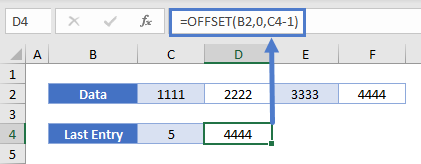
=OFFSET(B2,0,C4-1)