INDIRECT Sum – Excel & Google Sheets

This tutorial will teach you how to use the INDIRECT Function nested in the SUM Function in Excel and Google Sheets.

INDIRECT Sum Using Cell Reference

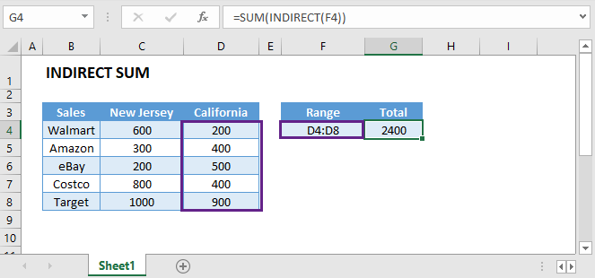
One way to sum a dynamically referenced range is by using a combination of the SUM and INDIRECT functions.

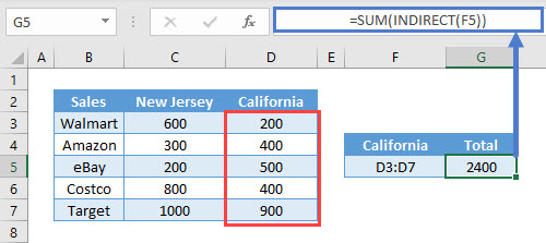
This example will SUM the defined range in cell F5.

=SUM(INDIRECT(F5))

INDIRECT Sum Using Dynamic Sheet Reference

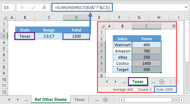
To sum a range dynamically referenced from another worksheet, use a similar formula:

=SUM(INDIRECT(B3&"!"&C3))

The difference here is that we also must define the sheet name.

INDIRECT – Volatile Function

Warning: The INDIRECT Function is volatile. This means it re-calculates every time the workbook re-calculates. If you rely on too many INDIRECT functions, it will negatively impact your workbook speed.

Alternatively, you can use other non-volatile functions. One such function is the OFFSET Function.

Dynamic SUM using OFFSET Function

The OFFSET Function returns a reference to a range that is offset from a starting cell or range by a specified number of rows and columns. It can be nested in the SUM Function to dynamically reference a range and sum values.

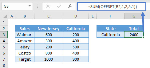
The following example uses the OFFSET Function to sum range ‘D3:D7‘.

=SUM(OFFSET(B2,1,2,5,1))

Starting with cell B2, the Function offsets one (1) row and two (2) columns to obtain the range D3:D7 with a height of 5 and width 1.

If the last two arguments ‘[height]‘ and ‘[width]‘ are omitted, the new reference will have the same height and width as the starting reference.

Note: The OFFSET Function allows formulas to dynamically adjust to the data. Therefore, an addition or deletion of rows and columns would not cause the final output to change.

INDIRECT Sum in Google Sheets

These formulas work exactly the same in Google Sheets as in Excel.