IFERROR (& IFNA) XLOOKUP

This tutorial will demonstrate how to handle XLOOKUP #N/A errors in Excel. If your version of Excel does not support XLOOKUP, read how to error handle VLOOKUPs instead.

XLOOKUP: #N/A Error-Handling

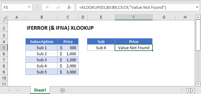
Unlike VLOOKUP, XLOOKUP has the built-in option to handle #N/A Errors. By entering a value into the 4^th argument, the XLOOKUP Function will replace a #N/A error with the specified value.

In this example, we replace the #N/A Error with the text “Value Not Found,”.

=XLOOKUP(E3,B3:B7,C3:C7,"Value Not Found")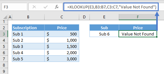

Or we can also set it to 0:

=XLOOKUP(E3,B3:B7,C3:C7,0)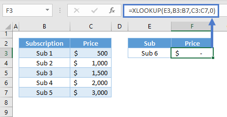

Note: The XLOOKUP Function requires at least three arguments: lookup value, lookup array and return array. By default, the XLOOKUP Function finds an exact match from the top of the lookup array going down (i.e., top-down). Once it finds a match, it returns the corresponding value from the return array. Otherwise, it returns an error.

Nested XLOOKUP: 2 Sheets at Once

Instead of a customized value, we can nest another XLOOKUP in the 4^th argument of the XLOOKUP Function to perform a lookup among multiple sets of data that are stored in different sheets.

=XLOOKUP(E3,B3:B7,C3:C7,XLOOKUP(E3,'2 Sheets - Data 2'!B3:B7,'2 Sheets - Data 2'!C3:C7))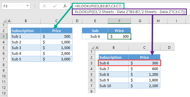

XLOOKUP & IFERROR

For arithmetic calculations involving XLOOKUP, we can use the IFERROR Function to handle all types of error.

=IFERROR(1.5*XLOOKUP(E3,B3:B7,C3:C7),"Value Not Found")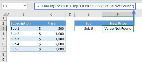

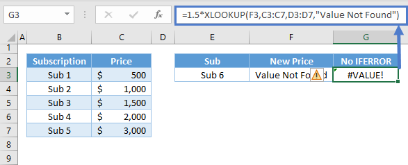
The #N/A Error handling of the XLOOKUP Function won’t work on the above scenario:

=1.5*XLOOKUP(F3,C3:C7,D3:D7,"Value Not Found")