Get Full Address of a Named Range in Excel & Google Sheets
Written by
Reviewed by
Download the example workbook
This tutorial will demonstrate how to get the full address of a named range in Excel & Google Sheets.
Named Ranges
A Named Range is a range of a single cell or multiple cells, which are assigned a specific name. Named Ranges are one of Microsoft Excel’s useful features; they can make formulae easier to understand.
Get Address of Named Range
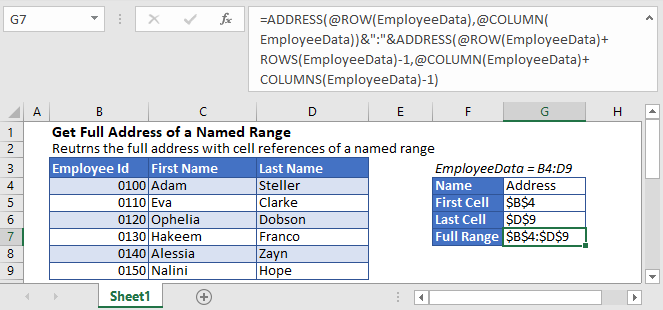
To get the full address of a named range, you can use an Excel formula that contains ADDRESS, ROW, ROWS, COLUMN, and COLUMNS functions.
In order to get the full address of a named range, we’ll find the first and last cell references of the named range and then join them together with a colon (“:”).
Get First Cell Address in a Named Range
Let’s say we have a named range “EmployeeData” in range B4:D9.
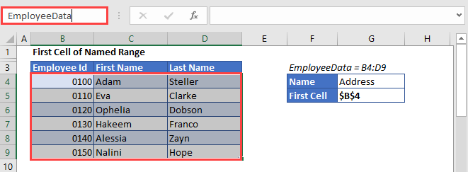
To get the cell reference of the first cell in a named range, we’ll use the ADDRESS function together with ROW and COLUMN functions:
=ADDRESS(ROW(EmployeeData),COLUMN(EmployeeData))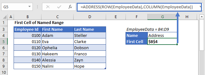
The ADDRESS function returns the address of a specific row and column. We use the ROW and COLUMN Functions to calculate the first row and column in the named range, plugging the results into the ADDRESS Function. The Result is the first cell in the named range.
The above formula has returned the absolute cell reference ($B$4). But if you want a relative address(without $ sign, B4), you need to supply 4 for the third (optional) argument of the ADDRESS function like this:
=ADDRESS(ROW(EmployeeData),COLUMN(EmployeeData),4)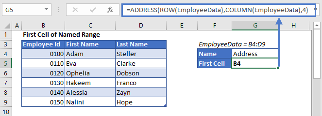
Get Last Cell Address in a Named Range
To get the cell reference of the last cell in a named range, we can use the following formula:
=ADDRESS(ROW(EmployeeData)+ROWS(EmployeeData)-1,COLUMN(EmployeeData)+COLUMNS(EmployeeData)-1)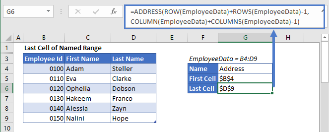
Here the ROWS and COLUMNS Functions count the number of rows and columns in the range, which we add to the original formula above, returning the last cell in the named range.
Similarly, if you want a relative address instead of an absolute cell reference, you can supply 4 for the third argument in the ADDRESS function like this:
=ADDRESS(ROW(EmployeeData)+ROWS(EmployeeData)-1,COLUMN(EmployeeData)+COLUMNS(EmployeeData)-1,4)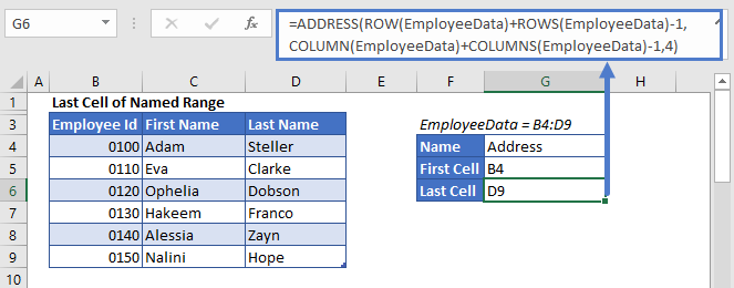
Full Address of Named Range
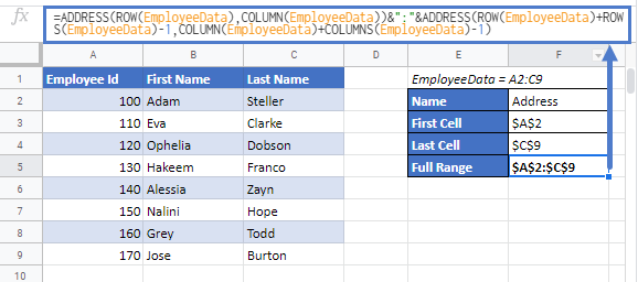
Now in order to get the complete address of a named range, we’ll just have to concatenate the above two formulas with the operator (:), in the above example like this:
=ADDRESS(ROW(EmployeeData),COLUMN(EmployeeData))&":"&ADDRESS(ROW(EmployeeData)+ROWS(EmployeeData)-1,COLUMN(EmployeeData)+COLUMNS(EmployeeData)-1)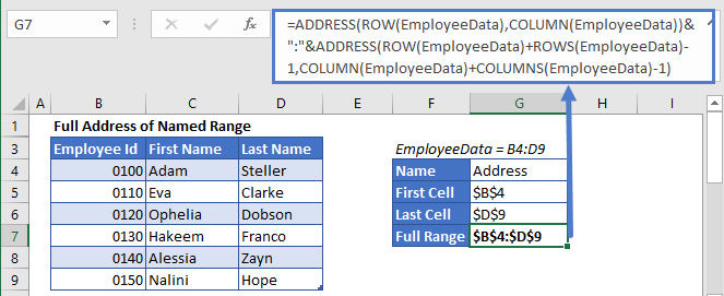
Similarly, to return the address of the named range as a relative reference (without $ sign), supply the third argument of the ADDRESS functions with 4, like this:
=ADDRESS(ROW(EmployeeData),COLUMN(EmployeeData),4)&":"&ADDRESS(ROW(EmployeeData)+ROWS(EmployeeData)-1,COLUMN(EmployeeData)+COLUMNS(EmployeeData)-1,4)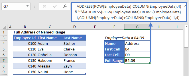
Get Full Address of a Named Range in Google Sheets
The formula to get the full address of a named range works exactly the same in Google Sheets as in Excel:
