Extract Text Between Characters (Parenthesis) in Excel & Google Sheets

Written by

Editorial Team

Reviewed by

Steve Rynearson

Last updated on February 7, 2023

Download Example Workbook

Download the example workbook

This tutorial will demonstrate how to extract text between characters in a cell in Excel & Google Sheets.

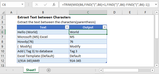
mf extract text between characters parenthesis

Extract Text Between Parenthesis

To extract the text between any characters, use a formula with the MID and FIND functions.

Use this formula to extract the text between parenthesis:

=MID(B3,FIND("(",B3)+1,FIND(")",B3)-FIND("(",B3)-1)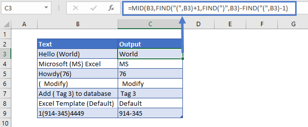

Extract Text Between Characters Formula

The FIND Function locates the parenthesis and the MID Function returns the characters in between them.

FIND Functions

The first FIND function locates the position of the left parenthesis “(“. Add 1 to the result to return the character immediately after the left parenthesis.

=FIND("(",B3)+1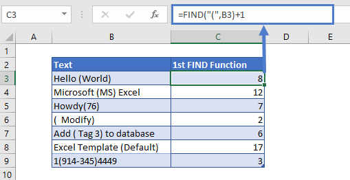

Extract Text Between Characters 1st Find Function

The second FIND function finds the position of the right parenthesis “)”.

=FIND(")",B3)

The third FIND function is subtracted from the second FIND function, returning the length of text between the parentheses.

=FIND(")",B3)-FIND("(",B3)-1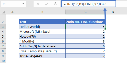

Extract Text Between Characters 2nd & 3rd Find Functions

MID Function

Both of these arguments’ values are entered into the MID function. This will give us the text between the parenthesis.

=MID(B3,C3,D3)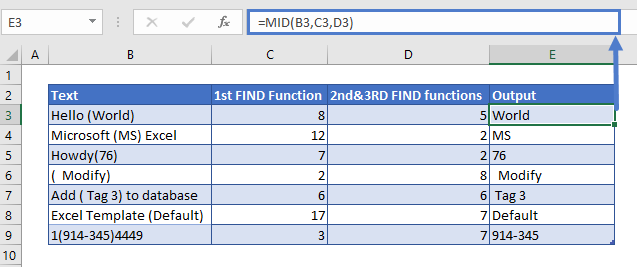

Extract Text Between Characters MID function

TRIM function

We can also add the TRIM Function before the MID function to remove all extra spaces.

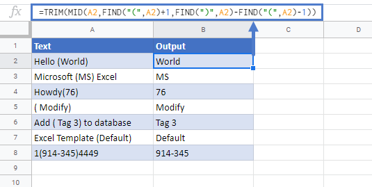
=TRIM(MID(B3,FIND("(",B3)+1,FIND(")",B3)-FIND("(",B3)-1))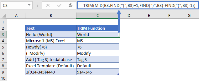

Extract Text Between Characters with Trim Function

Extract Text Between Characters In Google Sheets

The formula to extract text between characters works exactly the same in Google Sheets as in Excel:

Extract Text Between Characters in Google Sheets