Custom Sort List with Formula – Excel & Google Sheets
Written by
Reviewed by
Download the example workbook
This tutorial will demonstrate how to dynamically sort data by a custom sort order in Excel and Google Sheets.
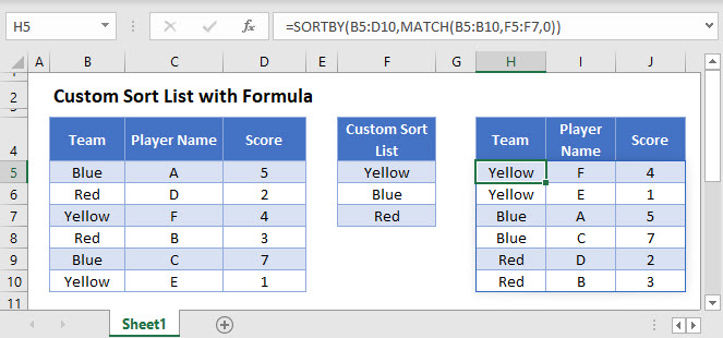
SORTBY Function in Excel 365
The SORTBY Function produces a dynamic array of sorted data.
In this example, we use the SORTBY Function to take a data table and produce a dynamic array that sorts it by Team following a Custom Sort List:
=SORTBY(B3:D8,MATCH(B3:B8,F3:F5,0))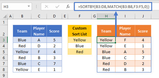
Note: The SORTBY Function is written in only cell H3. The rest of the table will populate automatically.
The sorted table is dynamic, which means that if any of the Team or Player Name values change or records or added / deleted, then the output table will automatically re-size and re-sort.
Note: The SORTBY Function is not available in Excel 2019 or earlier. Read below for sorting options available for earlier versions of Excel.
To explain how this formula works, let’s break it down into steps:
Our final formula is:
=SORTBY(B3:D8,MATCH(B3:B8,F3:F5,0))First, we define the data table that needs to be sorted. This will be B3:D8.
Next, we need to define the sort order. We will use the MATCH Function to find the order in which each Team name appears in the Custom Sort List. This part of the formula is:
=MATCH(B3:B8,F3:F5,0)Adding in the values from the cell ranges, we get:
=MATCH({"Blue"; "Red"; "Yellow"; "Red"; "Blue"; "Yellow"}, {"Yellow"; "Blue"; "Red"}, 0)The MATCH Function replaces all Team names with the order in which they appear in the Custom Sort List, using an exact text match:
={2; 3; 1; 3; 2; 1}This array of values is then used as the sort order by the main SORTBY Function:
=SORTBY(B3:D8, {2; 3; 1; 3; 2; 1} )The sorted table is then produced
Custom Sort List – Pre-Excel 365
As the SORTBY Function is not available to Excel users before the Excel 365 version, we will now show how to perform the same task using a more manual process.
The built-in Excel sort tool can be used to sort by a Custom Sort List by selecting the ‘Custom List…’ from the sort order options in the sort tool:
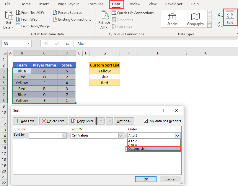
A new Custom List should be added as a comma separated list. In this example, we add: ‘Yellow, Blue, Red’
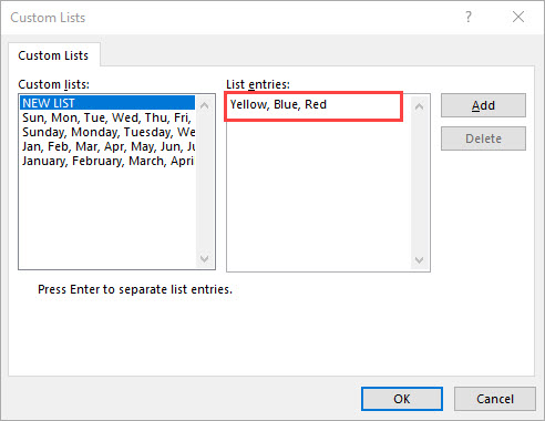
The Custom List is then shown in the sort order selection
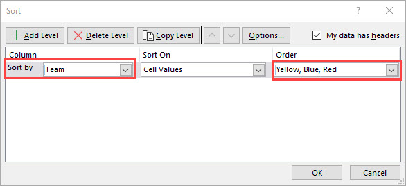
The data table is then sorted by the Custom List values
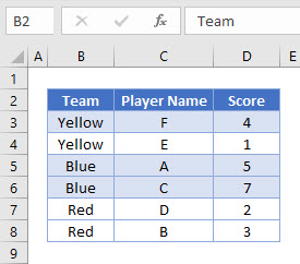
Note that this custom sort order is saved within the workbook and is available to be used again. If you do not wish to add a Custom List to Excel, then a method using a helper column can be tried instead.
Custom Sort List With Helper Column – Pre-Excel 365
In this next, example, we use the MATCH Function in a helper column to define a Custom Sort Order by referencing a Custom Sort List:
=MATCH(B3,$G$3:$G$5,0)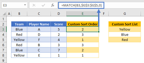
Note the use of the $ symbol when referencing the Custom Sort list. Please read our article on Locking Cell References to learn more on this subject.
One the helper column has been added, a manual sort process can be run using the Sort Wizard:

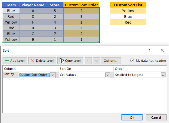
This then produces the table sorted following the Custom Sort Order:
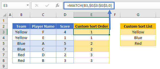
If any changes are made to the Team or Custom Sort List values, then the sort wizard will need to be re-run to update the sort order of the data table.
Custom Sort List with Formula in Google Sheets
The SORTBY Function is not available in Google Sheets, but its SORT Function can be used instead and is more powerful than the SORT Function in Excel 365. It allows us to use custom sort lists to dynamically sort data ranges.
In this example, we use the Google Sheets SORT Function to take a data table and produce a dynamic array that sorts Team values by a Custom Sort List:
=SORT(B3:D8,MATCH(B3:B8,F3:F5,0),TRUE)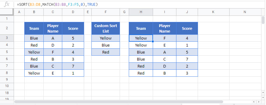
The Google Sheets SORT Function sorts data by the specified column numbers or custom sort orders in the input data and allows us to set whether the sort order is ascending or not


