Count If Multiple Criteria Excel and Google Sheets

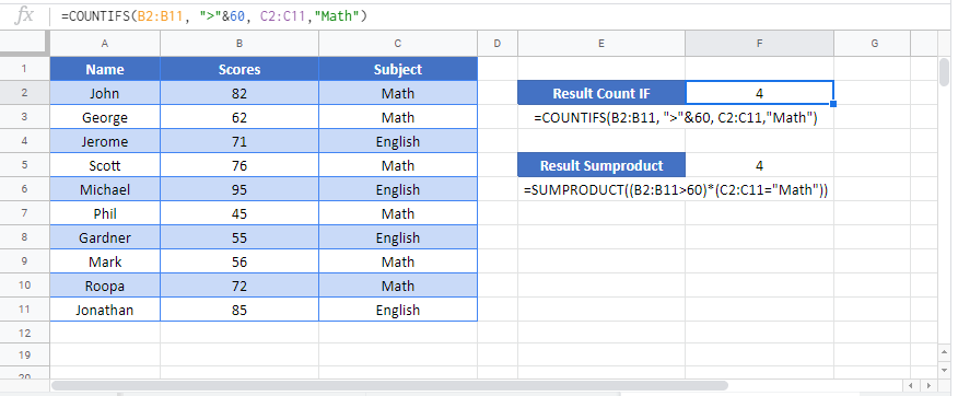
This tutorial demonstrates how to “count if” with multiple criteria using the COUNTIFS Function in Excel and Google Sheets. If your version of Excel does not support COUNTIFS, we also demonstrate how to use the SUMPRODUCT function instead.

COUNTIFS Function

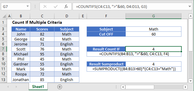
The COUNTIFS Function allows you to count values that meet multiple criteria. The basic formula structure is:

=COUNTIFS(Range 1, Condition 1, Range 2, Condition 2)

Let’s look at an example. Below you will see a list containing grades for students in English and Math. Let’s count all students with test scores above 60 in Math.

=COUNTIFS(C3:C12, ">"&60, D3:D12, "Math")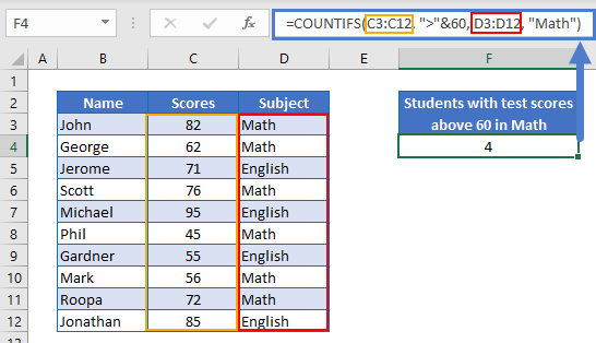

In this case, we are testing two criteria:

1. If the Test Scores are greater than 60 (Range B3:B12)
2. If the Subject is “Math” (Range is C3:C12)

Below, you can see that there are 4 students who scored above 60 in Math:

 

 

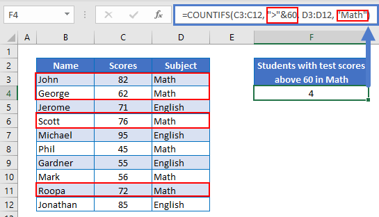
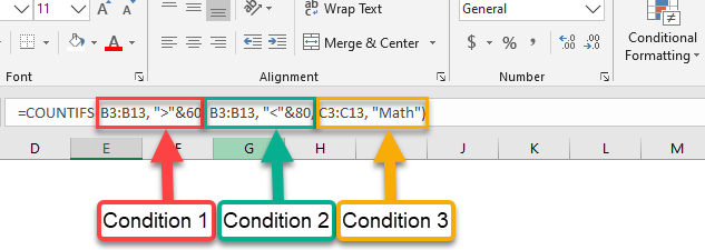
You can test additional conditions by adding another range and criteria.  For example, if you wanted to count the number of students who scored between 60 and 80 in Math you would use this criteria:

1. If the Test Scores are greater than 60
2. If the Test Scores are below 80
3. If the Subject is “Math”

Here are the highlighted sections where these examples are being tested.

The result, in this case, is 3.

=COUNTIFS(B3:B13,">" & 60,B3:B13,"<"&80,C3:C13,"Math")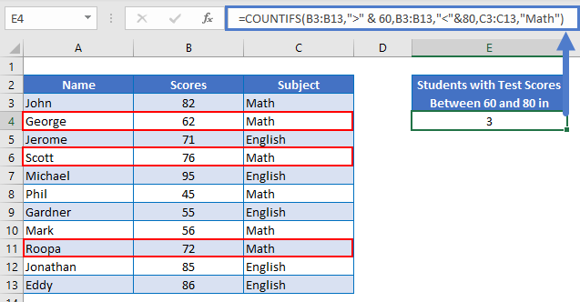

 

SUMPRODUCT Function

If you don’t have access to COUNTIFS, you can accomplish the same task with the SUMPRODUCT Function. The SUMPRODUCT Function opens up a world of possibilities with complex formulas (see SUMPRODUCT Tutorial). So, even if you have access to the COUNTIFS Function, you may want to start familiarizing yourself with this powerful function. It’s syntax is:

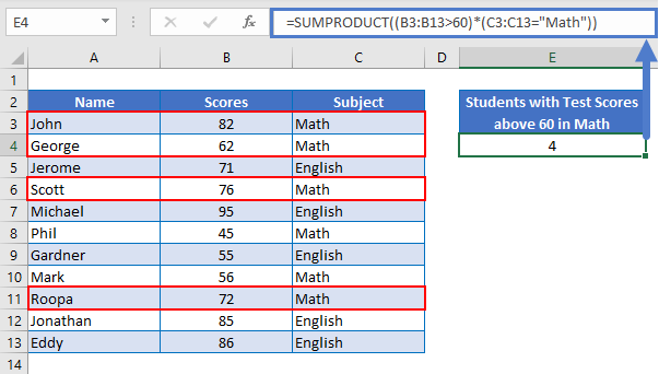
=SUMPRODUCT(Range 1=Condition 1*Range 2=Condition 2)

Using the same example above, to count all students with test scores above 60 in subject “Math”, you can use this formula:

=SUMPRODUCT((B3:B13>60)*(C3:C13="Math"))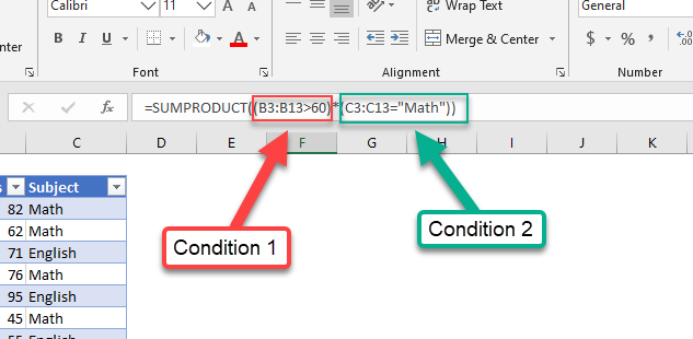

The first condition tests which values in that range are greater than 60, and the second condition tests which values in that range equal to “Math”. This gives us an array of Boolean values of 1 (TRUE) or 0 (FALSE):

=SUMPRODUCT(({82;62;71;76;95;45;55;56;72;85;86}>60)*({"Math";"Math";"English";"Math";"English";"Math";"English";"Math";"Math";"English";"English"}="Math"))

=SUMPRODUCT(({TRUE;TRUE;TRUE;TRUE;TRUE;FALSE;FALSE;FALSE;TRUE;TRUE;TRUE})*({TRUE;TRUE;FALSE;TRUE;FALSE;TRUE;FALSE;TRUE;TRUE;FALSE;FALSE}))

=SUMPRODUCT({1;1;0;1;0;0;0;0;1;0;0})

=4

 

The SUMPRODUCT Function then totals all items in the array, giving us the count of students who scored about 60 in math.

 

COUNTIFS and SUMPRODUCT for Multiple Criteria in Google Sheets

You can use the same formula structures as above in Google Sheets to count with multiple criteria.