Count if Cells in Range

This tutorial explains how to count the number of cells containing numbers that fall within a specified range using the COUNTIFS function.

COUNTIFS

COUNTIFS(range_1,criteria _1,[ range_2,criteria _2],…)

• range_1 (required): group of cells to count
• criteria_1 (required): conditions used to count
• range_2,criteria_2: optional ranges and criteria than can be evaluated. Up to 127 range and criteria pairs can be specified.

How COUNTIFS Works

The COUNTIFS function adds up the number of cells that fall within the ranges specified in the COUNTIF Function.

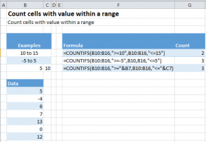
Let us see how to actually use the function. The following image shows COUNTIFS in action.

COUNTIFS Cells in Range Example Description

Let us now look at the formula and try to understand it, piece by piece.

1. In the first case, we call COUNTIFS in the following manner: =COUNTIFS(B10:B16,”>=10”,B10:B16 ,”<=15”)
   1. B10:B16 tells Excel the range over which we want to count
   2. “>=10”/ “<=15”, the criteria according to which we want to count the cells.
      1. “>=10″ stands for counting any value that is greater than or equal to 10
      2. “<=15” stands for counting any value that is less than or equal to 15
2. The second case is similar to the first case with only the counting criteria changing to
   1. “>=5”, greater than or equal to -5, i.e. -4,- 3, -2, -1, 0, 1…
   2. “<=5”, less than or equal to 5
3. The third case is a special case, one which we are very likely to face in a real life situation. This example shows us how to pick values like 5 and 10 from the spreadsheet rather than manually writing them in the formula. To achieve this, we call our function in the following manner: =COUNTIFS(B10:B16,”>=”&B7,B10:B16 ,”<=”&C7)
   1. The only thing changed in our function call as compared to before is our way of providing it our criterion, “>=”&B7/ “<=”&C7. The & sign followed by a cell number tells Excel to look at the value contained in the mentioned cell and use it to substitute it in the formula. Hence,
      1. The &B7 in “>=”&B7, tells excel to look for the value in the cell B7, which in our case is 5, and substitute it in our formula changing it into “>=5”
      2. Similarly &C7 in “<=”&C7 is translated by excel into “<=10”

COUNTIF Function

Before ending this tutorial, I would also like to talk a bit about the COUNTIF function.

Like COUNTIFS, COUNTIF can also be used to count the number of cells meeting specific criteria, but with one very important difference.

The difference between the COUNTIF and COUNTIFS functions is that while the latter function can be used to match multiple criteria in multiple ranges, the former can only match a single criterion in a single range. Multiple COUNTIF calls will be required to achieve this result.

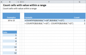
The image below shows how to find the count for the first case in above example using COUNTIF function:

EXPLANATION

The COUNTIF function is called as below:

= COUNTIF(B10:B16,”>=10″) – COUNTIF(B10:B16,”>15″)

The “>15” means all values greater than 15 will be counted but not 15 itself.

There are 3 operations happening over here

1. The first COUNTIF is counting all the values which are greater than or equal to 10
2. The second COUNTIF is counting all values that are strictly greater than 15
3. The final operation is subtracting the two counts found above in order to find our final count