Conditional Format Greater Than Or Less Than – Excel & Google Sheets

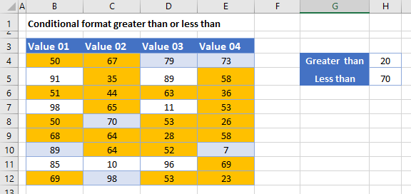
This tutorial will demonstrate how to highlight cells based on whether they are greater than or less than another cell using Conditional Formatting in Excel and Google Sheets.

 

 

Use a Highlight Cell Rule

To highlight cells where the value is greater than a specified number, you can use one of the built in Highlight Cell rules within the Conditional Formatting menu.

Greater Than

1. Select the range to apply the formatting (e.g., B4:E12).
2. In the Ribbon, select Home > Conditional Formatting > Highlight Cells Rules > Greater Than…

 

 

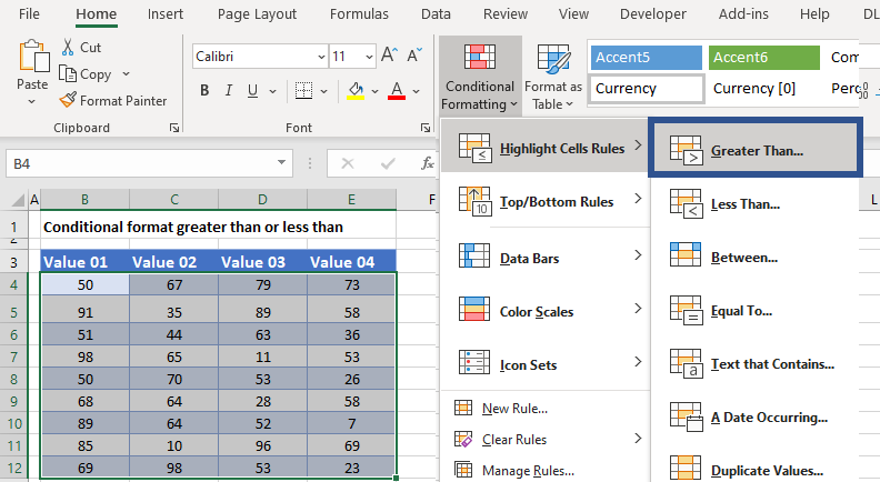
3. You can either type in the value, or to make the formatting dynamic (i.e., the result will change if you change the values), you can click on the cell that contains the value you require.

 

4. Select the type of formatting you require from the drop down box and click OK.

 

 

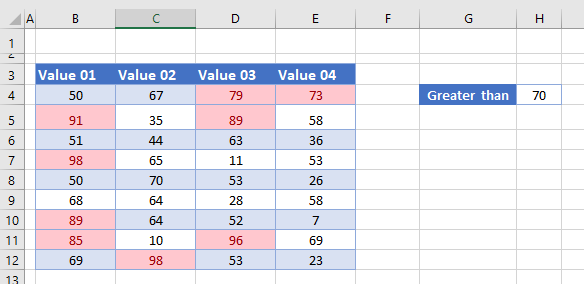
The table now indicates which values are greater than that in cell H4 (50) by making them red.

 

 

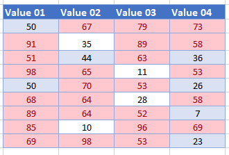
5. Change the value in H4 to obtain a different result.

 

 

Less Than

1. Select the range to apply the formatting.
2. In the Ribbon, select Home > Conditional Formatting > Highlight Cells Rules > Less Than…

 

 

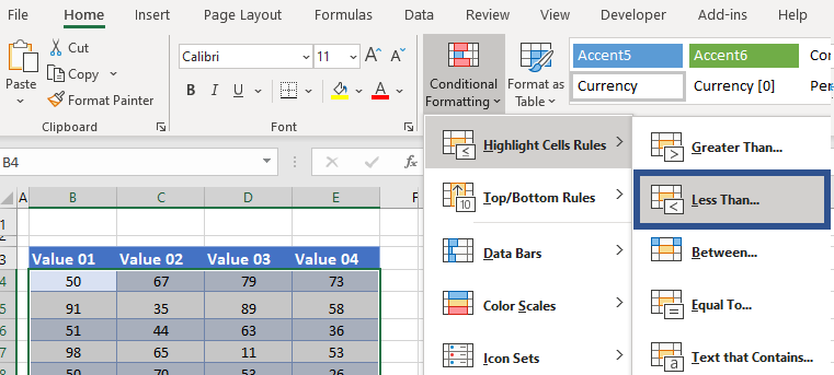
3. As before, click on the cell that contains the value you require.
4. Click OK to format the cells with the desired formatting.

 

 

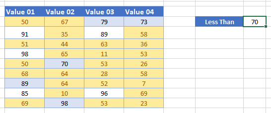
The resulting formatting shows numbers less than 70 in yellow.

 

Highlight Cells With a Custom Function

With Conditional Formatting, you can also highlight cells by using a custom function.

Greater Than AND Less Than

You can highlight cells that have a greater value than one cell, but a smaller value than another by creating a New Rule and selecting Use a formula to determine which cells to format.

1. Select the range to apply the formatting.
2. In the Ribbon, select Home > Conditional Formatting > New Rule.

 

 

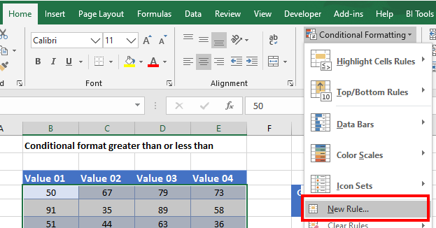
3. Select Use a formula to determine which cells to format, and enter this formula that uses the AND Function:

=AND(B4>$H$4, B4<$H$5)

 

4. You need to lock the reference to cells H4 and H5 by making them absolutes. Do this by using the $ sign around the row and column indicators, or by pressing F4 on the keyboard.
5. Finally, click on the Format button.

 

 

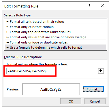
6. Select the formatting you want for numbers between H4 (20) and H5 (70). Click OK.

 

 

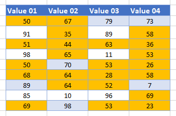
The result is similar to the previous examples, just highlighting on a different condition.

 

Greater Than OR Less Than

To highlight cells that have a greater value than one cell or have a smaller value than another cell (i.e., outside the range of the two cells), follow these steps:

1. Select the range to apply the formatting.
2. In the Ribbon, select Home > Conditional Formatting > New Rule
3. Select Use a formula to determine which cells to format, and enter this formula that uses the OR Function:

=OR(B4>$H$4, B4<$H$5)

 

4. Once again, lock the reference to cells H4 and H5 by making them absolutes. Use the $ sign around the row and column indicators, or press F4 on the keyboard.
5. Click on the Format button.

 

 

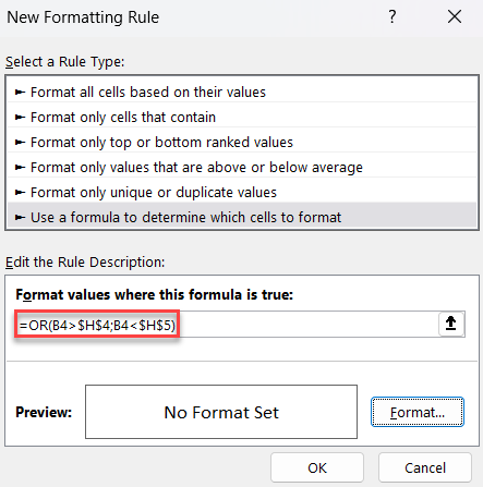
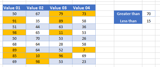
6. Select the formatting you want for numbers that are not between H4 (70) and H5 (15). Click OK.

 

 

Highlight Cells With a Custom Function in Google Sheets

The process to highlight cells with a greater value than one cell, and a smaller value than another cell in Google Sheets is similar to the process in Excel.

1. Highlight the cells you wish to format, and then click on Format > Conditional Formatting.
2. The Apply to Range section will already be filled in.

 

 

3. From the Format Rules section, select Custom Formula from the drop-down list and type in the following formula:

=AND(B4>$H$4, B4<$H$5)

 

 

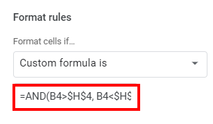
Once again, use the absolute signs (dollar signs) to lock in the values in H4 and H5.

4. Select the fill style for the cells that meet the criteria.

 

 

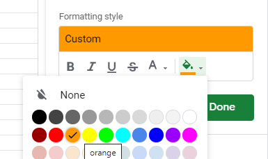
5. Click Done to apply the rule.