How to Edit Conditional Formatting in Excel & Google Sheets

This tutorial demonstrates how to edit conditional formatting in Excel and Google Sheets.

 

 

Edit Conditional Formatting Rules in Excel

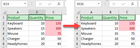
Using Rule Manager, you can easily change the hierarchy of conditional formatting rules, delete them, or make new ones.

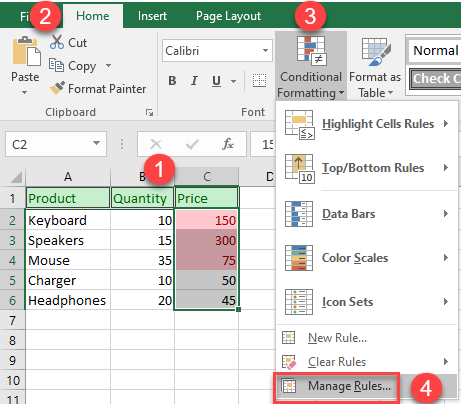
1. Select the data range (e.g., C1:C6).
2. In the Ribbon, go to Home > Conditional Formatting > Manage Rules…

 

 

3. In the Conditional Formatting Rules Manager window, select the rule you want to edit and click Edit Rule.

 

 

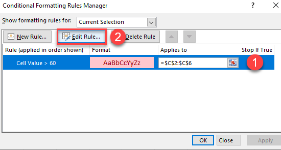
4. This opens the Edit Formatting Rule window. In it, you can choose a new rule type for a selected range or edit the existing rule.

 

 

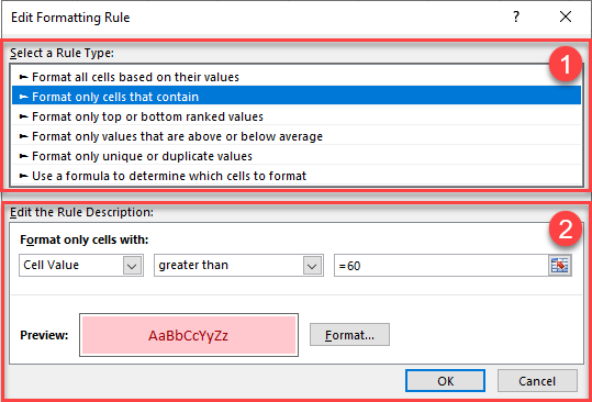
For more information on conditional formatting settings and options you can use to make your changes, see Conditional Formatting **Tips for 2022**.

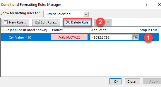
Note: To delete a rule, just select it and click the Delete Rule button.

 

 

Edit Conditional Formatting Rules in Google Sheets

In Google Sheets, you can edit an existing rule or simply update the format.

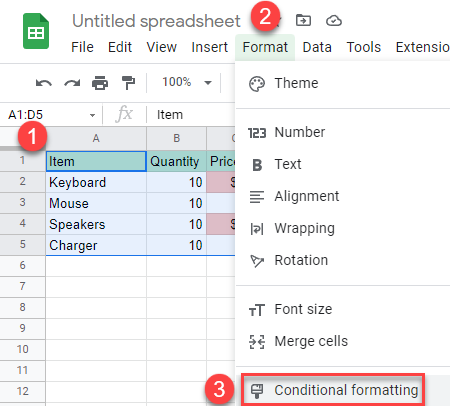
1. First, select the formatted range (e.g., A1:C5).
2. In the Menu, go to Format > Conditional Formatting.

 

 

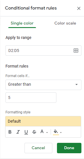
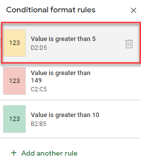
3. The Conditional format rules pane opens on the right side of the sheet. In it, double-click on the rule you want to edit.

 

 

4. Now, edit the rule and click Done.