Most Useful & Under-used Excel Functions
41 EXCEL EXPERTS WEIGH IN
Brought to You by AutomateExcel.com
Microsoft Excel has hundreds of functions. Even experienced Excel users can find themselves wondering if they are using the best Excel formulas for their projects.
With that in mind, we polled 41 Excel experts and asked them the question: What is the most under-used Excel function? Their answers are listed below.
Want to master the 30 most-used Excel Functions?
CHOOSE Function - 4 Votes
The CHOOSE function was my vote for the most under-used Excel function. It's easy to understand and very powerful. CHOOSE allows you to select one of up to 254 values or options based on an index number. - Michael from Excel Bytes.
As John from How to Excel implies, this might not sound like much, but in the right circumstance it can be very powerful: I remember when I first met CHOOSE. I thought to myself, "Wow, what a boring function. All it does is choose an item in your list based on an index number. Doesn't INDEX already do that?" It looks like a very simple function at the outset, but when you combine it with other formulas it can be quite powerful.
My favorite use of the CHOOSE Functions is this: Let's say you have 4 worksheets: a Forecast sheet, a Budget sheet, a Trailing 12 sheet, and a Summary sheet. On the Summary sheet, you use drop-downs to select which sheet's data to show:
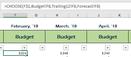
In the above example, the CHOOSE function allows you to read data from one of three sheets. Cell F$1 contains a MATCH function that looks to see what option was selected from the drop-down (drop-down currently reads "Budget") and returns the corresponding number, which is used by the CHOOSE function. You can see that by using the CHOOSE function you can select values from different sheets, while avoiding volatile functions like INDIRECT.
Lookup Formulas - VLOOKUP, HLOOKUP, INDEX, and MATCH - 5 Total Votes
The lookup functions are hands-down some of the most important Excel functions. You can't claim to be an Excel expert without being proficient with these.
VLOOKUP & HLOOKUP
Laurent from ExcelMadeEasy says this about the Vlookup: Looking for data in a specific column, row, or a full table? Excel has a solution in the form of VLOOKUP and HLOOKUP functions.
The VLOOKUP allows you to search for a value in a column ("V" for vertical) and return another value from that same row. The HLOOKUP allows you to search for a value in a row ("H" for "horizontal") and return another value from that same column.
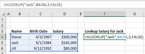
The VLOOKUP and HLOOKUP have two big limitations:
- The lookup column must be the left-most column in the data (or top-most row for a HLOOKUP). Often your data will not come in this format.
- In large workbooks, these lookup functions can take a very long time to run. Ole from Erlandsen Data Consulting says this: A little bit off-topic, but here is a function that I think is sometimes over-used or used in a wrong way: VLOOKUP. This function is extremely useful, but can sometimes cause the calculations in a workbook to slow down to a crawl when used with large data sources and/or in a lot of cells. An example: a workbook that took 5-10 minutes to calculate because of excessive use of the VLOOKUP function, took 7 seconds to calculate after sorting the data sources and replacing VLOOKUP with MATCH and INDEX functions.
NDEX & MATCH
The MATCH function looks up a value in an array of cells and returns the position # where that value is found.
The INDEX function returns a value from an array of cells based on the provided position #.
Together these functions can be used to simulate a VLOOKUP, only with more flexibility. Othniel from Excellent Ones Consulting says this These two functions together are more powerful than the traditional VLOOKUP In a VLOOKUP formula the field to be matched must be in the first column of your data set. Using a combination of Index and match removes those limitation. This adds more flexibility to the user.
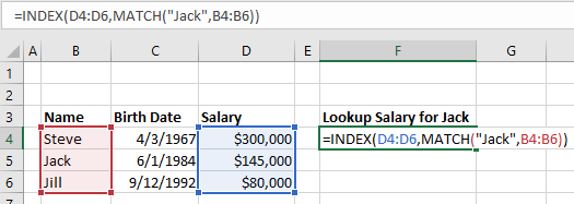
Alan from ComputerGaga notes some other advanced uses of the INDEX function: However other awesome uses include to return the last value from a row or column, to create dynamic ranges and its use with form controls for interactive charts and dashboards.
Match Multiple Criteria with a Formula
These functions also allow you to match multiple criteria. However, the formula is quite complicated!
Marcus Small explains My favourite function to rip out in any of my courses is the combination of INDEX, MATCH, and INDEX. This powerful three part formula allows you to return a match based on multiple criteria. It avoids the concatenation of data with the inevitable use of VLOOKUP and it does not need to be in the form of an array formulation. One caveat, I only use this formula when I am wanting to return TEXT based on multiple criteria, as Excel has SUMIFS and SUMPRODUCT available to deal with multi criteria calculation returns. Quite simply it is formulaic brilliance!!!
The syntax is
Index(result column, match(1, index((criteria range=criteria)*(criteria range2 =criteria2),0),0))
The formula works as it is attempting to match the true condition to the specified criteria. In the above example there is 2 criteria however you could have 3, 4, 5 etc. The secret lies in the 1 part of the MATCH formula. If a match is made in the second INDEX, Excel produces a 1, if no match to the corresponding cell in the second INDEX criteria, Excel produces a zero, so 1 x 0 = 0. Excel continues until 2 matches are made 1 x 1 = 1 and the row where this occurs is then pushed into the first INDEX formula (INDEX(Result Column) to return the value of the row in the result column. It is a marvellous formula which can easily be extended with little effort. Here is 3 criteria:
Index(result column, match(1, index((criteria range=criteria)*(criteria range2 =criteria2)*(criteria range3 =criteria3),0),0))
Now the structure of a file can be preserved without resorting to adding a column to concatenate data so it can be used as LOOKUP criteria.
IFERROR Function - 3 Votes
IFERROR was one of my top choices for the most under-used function in Excel. It's easy to use, and makes your spreadsheets look much more professional.
Janet from Savvy Spreadsheets describes it's usefulness: I've seen too many reports with ugly # errors in them. The IFERROR function can be wrapped around a formula to quickly and easily hide those errors, by returning something else such as a blank or zero.
If you submit a spreadsheet to a client or superior filled with formula errors, it makes you look bad. Did you even review those errors? Are they valid errors or not? IFERROR makes a huge difference in how the quality of your work is perceived.
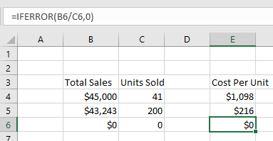
Joe from Excel by Joe describes how to use it: IFERROR is very easy to set up and it can easily eliminate all error messages from your function results. I use it all the time when building spreadsheets. To use it, simply insert whatever function you have written into the first part of the IFERROR and then put a comma and then enter what you want shown if there's an error. For example, if you want to display a zero whenever your function, A1/A2 has an error, use this code : =IFERROR(A1/A2,0)
Zach from Data Automation Professionals notes that IFERROR was a new function for Excel 2007. Microsoft added this function to save you the hassle of using =IF(ISERROR( and needing to enter the same formula twice.
SUMPRODUCT Function - 3 Votes
The SUMPRODUCT Function sums the products of multiple arrays. The simplest example is calculating total sales revenue based on # of Units Sold and Price per Unit:

SUMPRODUCT can also be used to perform advanced calculations. By creating columns with 1 or 0, you can create "if" conditions where records are only counted if they meet certain criteria (note: multiplying by 0 excludes the record from the SUMPRODUCT, multiplying by 1 includes it). As Ashish says, SUMPRODUCT allows one to specify multiple AND/OR conditions. My Excel Online notes that: this technique is like using SUMIFS on steroids.
Glen from Need a Spreadsheet is right when he says, It takes a while to get your head around SUMPRODUCT, but when you do it gives you enormous power and flexibility.
CONCATENATE, CONCAT, & TEXTJOIN Functions - 2 Votes
Juan from Excel MOOC and Mourad from Excel-Translator voted for CONCATENATE / CONCAT. The CONCATENATE function merges strings of text together. The CONCAT function is a newer version that does the same thing except with a shorter name (less typing the better!). Here is an example of merging text with a space (" ") in between:
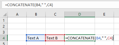
The big downside to CONCATENATE is that you can't merge an array of cells together. Instead, you must manually select each cell to merge. Microsoft fixed this problem with the new (for Excel 2016) function: TEXTJOIN:
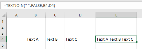
Notice the syntax: First you enter the deliminator (we chose a space " "). Next you enter TRUE/FALSE to decide if blank cells are counted, and last you enter the range to merge.
SIGN Function - 2 Votes
From Amiq Khan's blog: The Excel SIGN function checks the sign of a number and gives result of 1 if the number is positive, 0 if number is zero and -1 if the number is negative.
When would you use this?
Bill Jelen is a big fan of using the SIGN Function with the Up/Flat/Down icon set:

Bill says: In Row 1, negative numbers like -24 in I1 get an up indicator. Use the SIGN Function to make sure you only get 1,0, or -1 and the icons behave.
SUMIFS & More - 2 Votes
Alex Powers from It's Not About the Cell and Joseph from Spreadsheets Made Easy both voted for the SUMIFS, COUNTIFS, and, AVERAGEIFS Functions. These functions allow you to perform the desired calculations (sum, count, or average), only on data that meet certain criteria.
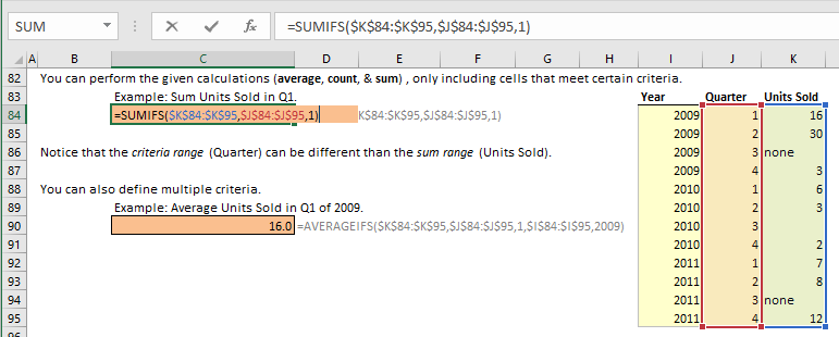
Also, new for Excel 2016 are the MAXIFS and MINIFS Functions (a life-saver for some of the work that I've done).
Alex and Joseph also noted that you can transform the basic SUM Function into a much more powerful SUMIFS with the use of "array" functions. Array functions are sometimes referred to as CSE (CTRL + SHIFT + ENTER) functions because when you enter the functions you must type CTRL + SHIFT + ENTER. With array functions, you can perform very complicated calculations, however they can be hard to create (or follow) for all but the most advanced Excel users. With that in mind, we won't cover an example.
TEXT Function - 2 Votes
The TEXT Function allows you to display a number stored as text in a specified number format.
Brad Edgar described this example: In cell A1 you have the date 04-OCT-2017 and you want to reference that date in a string of text:
="Today's date is: " & A1
By default, Excel will show "Today's date is: 43012" (43012 is the serial number corresponding to that date). Instead, to show the nicely formatted date use the TEXT Function:
="Today's date is: " & TEXT(A1,"DD-MMM-YYYY")

Steve=True from Excel Dashboard Templates had another example:
If you want to display a number with leading zeroes (ex. a ZIP code):

IF and IFS (New for Excel 2016) - 2 Votes
The IF function is ubiquitous in all of coding, as Alex discusses here. It tests if a condition is met. If so, it does something, if not it does something else. You won't get very far with Excel (or any coding language) without understanding this common function.
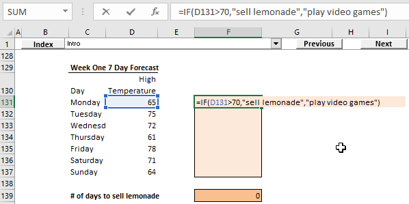
New for Excel 2016, Microsoft released the IFS function. Nick from Excel Spreadsheet Help says: With the IFS function you can now simplify one of the most common uses of the IF function: the dreaded nested IFs. If you use Excel frequently then at some point you’ve probably had to create a crazy long formula with multiple IF functions where it’s difficult to keep track of all the logic and commas. With the release of Excel 2016, the IFS function provides the same results as a nested IF formula but with a much simpler and easy to read method. IFS may be one of the most under-used Excel functions for now because it’s so new, but I think it’s use is going to spread rapidly once Excel users are aware of it existence!
Become an Excel Function Expert
Take our 100% free interactive tutorial on Excel functions. Master the 30 most-used Excel functions!
CONVERT - 2 Votes
From Charlie at Engineer Excel: CONVERT is a really efficient way to convert many different quantities like length, mass, volume, etc. between different sets of units. I find that many people (myself included before I found this function) "hard code" numbers into their spreadsheets in order to convert between unit systems. The CONVERT function eliminates the need to do that.
Kawser from Exceldemy provides a good example: Say I want to convert 100 Tones to Stones. See the image below.
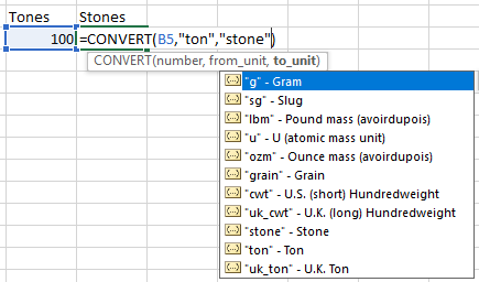
It's easy to convert almost any unit to other relevant unit using this Excel function.
SUBTOTAL Function - 1 Votes
Ben from Excel Exposure voted for the SUBTOTAL function saying: People generally don't know what it does, or how to use it. Even while praising it now myself, I realize I don't use it enough.
The SUBTOTAL Functions allows you to perform different calculations on a data set. You can see the list of options when you enter the function into Excel:
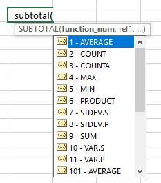
You might be asking yourself, why wouldn't you just use the AVERAGE function if you want to average or the COUNT function if you want to count?
You would use SUBTOTAL when you might change which calculation you wish to view. For example, you create a summary sheet to summarize a very large data set. You create a drop-down to select what information to show. Without using the SUBTOTAL function, you would need to create each calculation individually, and the drop-down would select which to show. With SUBTOTAL, you can create one formula that reads the drop-down and performs the appropriate calculation.
The SUBTOTAL function can reduce your calculation speed and reduce the number of formulas needed.
DOLLARDE and DOLLARFR - 1 Votes
Vijay from E for Excel says: Though designed as financial functions, these perform great conversion routines. I, very often, use them for time to decimal conversions. For example, 1:30 hours is 1.5 hours in decimal.
=DOLLARDE(1.30,60)
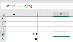
To convert it back to 1:30
=DOLLARFR(1.5,60)
(Note, it converts decimals not time value i.e. why 1.3 has been used to convert into 1.5. Though the same you can achieve through multiplying by 24 in case of DOLLARDE and divide by 24 for DOLLARFR. Hence 1:30/24 will give 1.5 and 1.5/24 will give 1:30)
The impact is even more strong once you perform other odd conversions
Convert 6 feet 6 inches
=DOLLARDE(6.06,12)
Which is 6.5 i.e. 6 and half feet
Similarily 6.3 is 6.5 dozen if =DOLLARDE(6.5,6) i.e. 6 and half dozen
So, you can perform many odd conversions which can not be done by CONVERT function.
Date Functions - 1 `Votes
Erin from Time Saving Templates suggested the date functions: DAY, MONTH, and YEAR. These functions extract the day, month, or year number from a date. If you work with dates you should know and use these (easy to remember) functions.
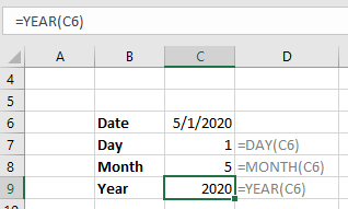
I also recommend the EDATE, EOMONTH, and DATE Functions. EDATE and EOMONTH roll dates forward or back a number of months (EOMONTH then returns the last day of that month). DATE is used to create a date from a given day, month or, year.
When entering dates into Excel, use one input cell to provide the starting date or year, and calculate all other dates using these functions. This makes updating spreadsheets monthly or annually a breeze! No more manually editing hard-coded dates!
MMULT Function - 1 `Votes
Earlier we mentioned the SUMPRODUCT function. SUMPRODUCT allows you to sum the products of multiple arrays. The MMULT function can be used in a similar way. Oscar from Get Digital Help says MMULT allows you to do calculations like the SUMPRODUCT function but in a more granular way. SUMPRODUCT lets you multiply and then sum arrays, whereas the MMULT function lets you multiply and sum arrays row-wise or column-wise.
MMULT stands for Matrix Multiplication. If you have a strong math background, you'll know exactly what it does:
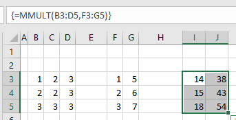
It's also an Array function (notice the brackets surrounding the formula above), which means you must use CTRL + SHIFT + ENTER when entering the formula.
INDIRECT Function - 1 `Votes
Abhilash from Excel to XL recommended the INDIRECT function. The INDIRECT Function allows you to "indirectly" reference cell ranges by treating the cell range as text.
To reference cell A1:
=INDIRECT("A1")
This is useful when you want to use formulas to determine which cell to reference. So instead of hard-coding "A1" into the formula above, you could reference a cell with formulas that output "A1", "B2", etc. This can be VERY useful when your desired ranges are on different worksheets.
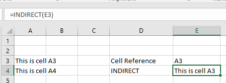
Warning: INDIRECT is a "volatile" function, meaning it re-calculates every time Excel recalculates the workbook. They won't slow your workbook down if you use a small number of them, but if you have large blocks of INDIRECT functions, you may start to notice a lag.
Often, you can avoid INDIRECTs with smart use of the CHOOSE and INDEX functions (see above).
LEN Function - 1 `Votes
The LEN Function counts the number of characters in a string of text. LEN can be useful when using other text functions such as LEFT, RIGHT, or MID.
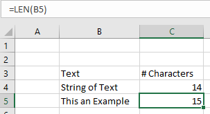
Onur from Someka.net makes an outstanding point about using LEN to check for blank cells: LEN is the most reliable way to check blank cells.
Some of you may ask: "Hey, I use =IF(A1="",...) method for checking blank cells, why would I need the LEN function? Aren't they the same?"
I prefer to use LEN for two reasons:
- When you copy and paste from other applications (word, access) blank cells are not counted as "real blank cells". (read more)
- Sometimes people enter space, line break, dot, or something similar to a blank cell, whether intentionally or accidentally. The workbooks need to account for this as well.
For these reasons to be on the very safe side I prefer to use LEN. In most cases, =IF(A1="",...) will do the work though.
OFFSET Function - 1 `Votes
Ismael from Excelforo voted for the OFFSET function. With the OFFSET function, you reference a cell by "offsetting" a certain number of rows and columns from a starting point. You can also resize the cell range to any number of rows and columns.
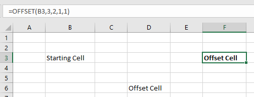
I've found the OFFSET function be extremely useful when coupled with VBA code that inserts and deletes rows and columns. By using the OFFSET, you can avoid #REF errors that appear when referenced cells are deleted.
Note: OFFSET is a "volatile function". Volatile functions recalculate each time Excel recalculates. If you have too many OFFSET functions, your workbook will slow down.
REPT Function - 1 `Votes
The REPT function allows you to repeat a string of text a certain number of times:
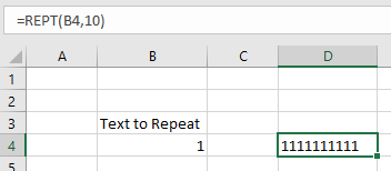
The true value of this function, however, lies in more creative uses as Crispo from CrispExcel points out: Although classified as a text function, REPT function does more than just repeating texts a number of times. For example, REPT is a perfect alternative to the slow calculating and complex Nested IF function. This is because REPT function can also act as a Logical Function returning an empty string if the number to return is zero. This ability to return an empty string makes it a perfect function for leaving comments within a cell instead of using N function.
REPT's ability to repeat characters also makes it perfect to create Mirror Charts (see below), Inline charts, Stem & Leaf Plots, Sparkline, star rating template and even the elusive FOMC dot plot chart.
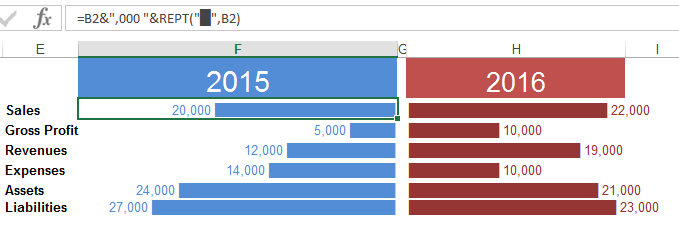
Mirror Chart
CELL & GET Functions - 1 `Votes
The team at Spreadsheet Detective suggested the GET & CELL functions. The GET function is an old XL4 function that can't be used in the same way as a normal Excel function. If you're interested in using this function, here is more information (warning: It's complicated).
The function can return useful information about a cell: color, row height, and much more. However, all of this can also be accomplished using VBA or some of the functionality can be accomplished with the newer CELL function.
The CELL function can return the following information about a cell:
Simply define the information you want to see and which cell you want to test!
MOD Function - 1 `Votes
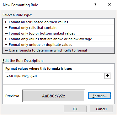
The MOD function returns the remainder of two numbers after division. Why is this useful? You can easily determine odd or even numbered rows (for alternate row shading) and, more generally, split data into separate groups.
Jorge from Power Spreadsheets says: The main reason I find MOD useful is because of how it allows you to break a group of items into different groups. I commonly use MOD in 2 contexts: (i) in conditional formatting formulas, such as formatting alternate rows or columns; or (ii) to classify entries or values into different groups, which allows you to work with subsets or them (for example, working with odd or even numbers, or entries located every nth cell).
GETPIVOTDATA - 1 `Votes
Debra from Contextures.com recommended the GETPIVOTDATA function: A GETPIVOTDATA formula is automatically created if you link to a PivotTable Value cell. Don’t turn that feature off! Learn how to tweak the formula, so it will pull out the pivot table data that you need.
Her site has an excellent page on the GETPIVOTDATA Function. Visit it to learn more.

User-Defined Functions - 1 `Votes
User-Defined Functions (UDFs) are custom functions created in VBA. If Excel doesn't have a function that you need, you can create your own in VBA. Obviously, VBA isn't for everyone, but if you are familiar with VBA, you might want to keep UDFs in mind. Jon from Vertex42 talks about UDFs: I think that custom user-defined functions may be underutilized. While there are many reasons why you might not want to use VBA within a spreadsheet, it is pretty simple to create your own add-in and populate it with custom functions that help speed up what you do in Excel. I avoid using custom functions in spreadsheets that I share with other people, but there are many custom functions that I use that allow me to easily do things I might not otherwise be able to do. Using the VB date functions to work with dates prior to 1900 is an example.
Text to Columns - 1 `Votes
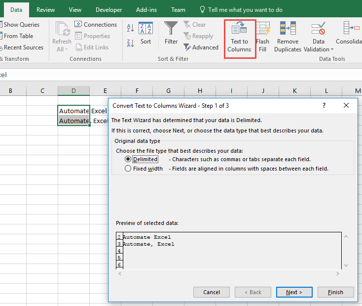
Text to Columns isn't an Excel function, but it is a very powerful Excel tool that can be used instead of using Excel text functions. The team at TestsTestsTests.com says this: Excel users (that don't know better) can spend hours manually separating and moving data from a single column to adjacent columns using copy/cut and paste or Excel text functions like LEFT, RIGHT, MID, etc.. A column may contain names, surnames, and/or dates of births that needs to be separated. A surprisingly quick and easy way of doing this is to use Text to Columns located in the Data Tools group under the Data tab of the Excel Ribbon. Text to Columns provides multiple options to separate the data, including by delimiters such as spaces or commas, or by a fixed width, allowing you to separate the data visually. This tool becomes especially useful when data is copied and pasted from other applications, such as tables in Microsoft Word, .csv (comma separated values) files, and more.
Flash Fill - 1 `Votes
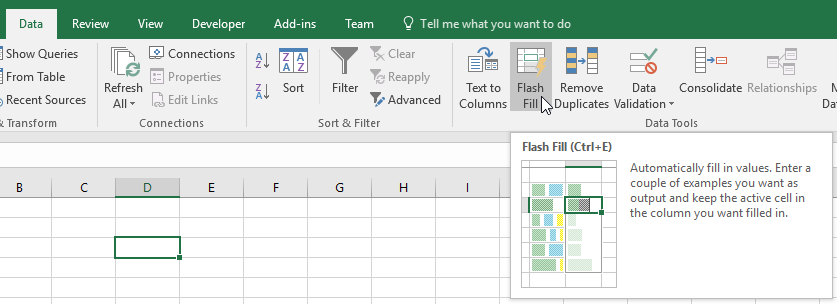
Just like Text to Columns, Flash Fill isn't an Excel function, but it is an under-used feature of Excel that can help alleviate the need for complex Excel formulas. The team over at Yoda Learning said this: Simply enter a pattern in the first several cells. Go to Data > Flash Fill (CTRL + E) and Excel will calculate the algorithm for the rest of the column.
Note: Generally, you would use this when you have a column of fully-populated data and you would like to create a second column based off of the first. For example, in the second column you would like to add "test" in front of the text from the first column. Instead of creating a formula to do so, you would manually enter the values in and then go to Flash Fill to populate the rest of the column.
You might notice that Excel suggests this automatically for you. In the Options menu you can toggle whether automatic Flash Fill is enabled or not.
Become an Excel Function Expert
Take our 100% free interactive tutorial on Excel functions. Master the 30 most-used Excel functions!
