UPPER Function Examples – Excel & Google Sheets
Written by
Reviewed by
Download the example workbook
This tutorial demonstrates how to use the UPPER Function in Excel to convert text to upper case.
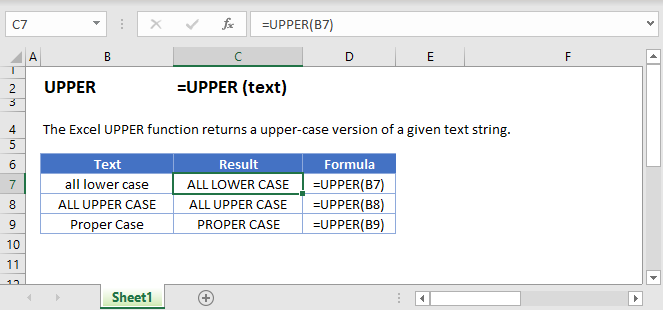
What Is the UPPER Function?
The UPPER Function takes a string as an input, and then returns the same string in upper case.
How to Use the UPPER Function
Use the Excel UPPER function like this:
=UPPER(“usa”)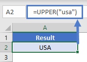
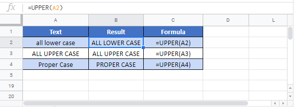
See below for a few more examples:
=UPPER(A2)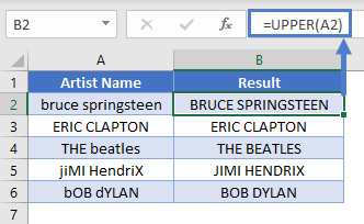
How UPPER Handles Numbers and Special Characters
The Excel UPPER Function has no effect on numbers, punctuation marks, or other special characters.
How UPPER Handles Accented Letters
Generally speaking, if you use UPPER on a text string that contains lower case, accented letters, Excel will return an accented capital if one exists. However, UPPER is somewhat intelligent in how it goes about this.
See the following examples:
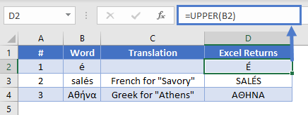
In examples #1 and #2, we see that Excel capitalizes the accented letter whether it is alone or part of a word. This is worth keeping in mind, as in some language like French and Portuguese, upper case letters are sometimes not accented, depending on the style guide being followed.
In Greek, where words that appear entirely in upper case should not be accented, UPPER does not accent the capitalized letters, as you can see in examples #3, where ή is correctly transformed to H, not its accented version Ή.
Using UPPER to count characters within a cell regardless of case
Say you need to count the number of times a particular character appears in a string, but you don’t care whether it’s upper or lower case. To do this, you can combine UPPER with LEN and SUBSTITUTE.
Look at these examples:
=LEN(B2)-LEN(SUBSTITUTE(B2,C2,""))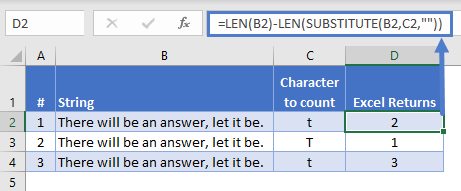
In example #1, we use LEN to count the number of characters in B2 – which happens to be 35 characters.
Then, we use SUBSTITUTE to go through B2, look for any character that matches whatever’s in C2 – in this case, a lower-case t – and replace them with an empty string. In effect, we remove them. Then we pass the result to LEN, which happens to be 33.
The formula is subtracting the second calculation from the first: 35 – 33 = 2. This means a lower-case t appears in the B2 twice.
In example #2, we’ve done the same thing, but we’re looking for an upper-case T – and we find one.
But if we want to find upper OR lower case Ts, we need to use UPPER. You can see this in example #3 – within the substitute part of the formula, we convert both B4 and C4 to upper case – so this time, we find three matches.
UPPER in Google Sheets
The UPPER Function works exactly the same in Google Sheets as in Excel: