HLOOKUP Function Examples in Excel, VBA, & Google Sheets

This tutorial demonstrates how to use the HLOOKUP Function in Excel and Google Sheets to look up a value.

 

What is the HLOOKUP function?

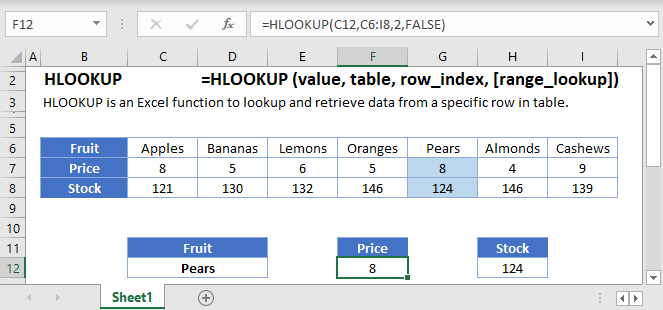
The HLOOKUP function is used to perform Horizontal Lookups (as opposed to VLOOKUPs which perform Vertical Lookups). It searches for a value in the top row of a table. Then returns a value a specified number of rows down from the found value.

It has a few limitations that are often overcome with other functions, such as INDEX / MATCH or XLOOKUP.

HLOOKUP – Basic Example

Let’s look at a sample of data from a grade book. We’ll tackle several examples for extracting information for specific students.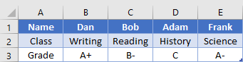

If we want to find what class Bob is in, we would write the formula:

=HLOOKUP("Bob", A1:E3, 2, FALSE)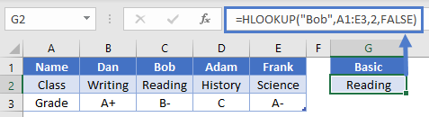

Important things to remember:

• The item we’re searching for (Bob), must be in the first row of our search range (A1:E3).
• We’ve told the function that we want to return a value from the 2^nd row of the search range, which in this case is row 2.
• We indicated that we want to do an exact match by placing False as the last argument. Here, the answer will be “Reading”.

Side tip: You can also use the number 0 instead of False as the final argument, as they have the same value. Some people prefer this as it’s quicker to write. Just know that both are acceptable.

Let’s review the Syntax:

HLOOKUP Function Syntax and Input:

=HLOOKUP(lookup_value,table_array,row_index_num,range_lookup)

lookup_value – The value you want to search for.

table_array -The table from which to retrieve data.

row_index_num – The row number from which to retrieve data.

range_lookup -[optional] A boolean to indicate exact match or approximate match. Default = TRUE = approximate match.

HLOOKUP – Shifted Data

To add some clarification to our first example, the lookup item doesn’t have to be in row 1 of your spreadsheet, just the first row of your search range. Let’s use the same data set:

Now, let’s find the grade for the class of Science. Our formula would be

=HLOOKUP("Science", A2:E3, 2, FALSE)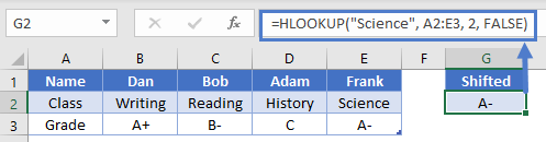

This is still a valid formula, as the first row of our search range is row 2, which is where our search term of “Science” will be found. We’re returning a value from the 2^nd row of the search range, which in this case is row 3. The answer then is “A-“.

Wildcards

The HLOOKUP function supports the use of the wildcards “*” an “?” when doing searches. For instance, let’s say that we’d forgotten how to spell Frank’s name, and just wanted to search for a name that starts with “F”. We could write the formula

=HLOOKUP("F*", A1:E3, 2, FALSE)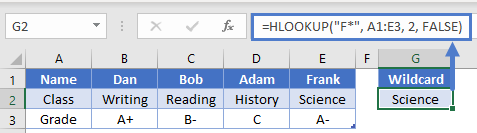

This would be able to find the name Frank in column E, and then return the value from 2^nd relative row.  In this case, the answer will be “Science”.

Non-Exact Match

Most of the time, you’ll want to make sure that the last argument in HLOOKUP is False (or 0) so that you get an exact match. However, there are a few times when you might be searching for a non-exact match. If you have a list of sorted data, you can also use HLOOKUP to return the result for the item that is either the same, or next smallest. This is often used when dealing with increasing ranges of numbers, such as in a tax table or commission bonuses.

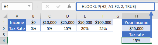
Let’s say that you want to find the tax rate for an income entered cell H2. The formula in H4 can be:

=HLOOKUP(H2, B1:F2, 2, TRUE)

 

The difference in this formula is that our last argument is “True”. In our specific example, we can see that when our individual inputs an income of $45,000 they will have a tax rate of 15%.

Note: Although we usually are wanting an exact match with False as the argument, it you forget to specify the 4^th argument in a HLOOKUP, the default is True. This can cause you to get some unexpected results, especially when dealing with text values.

Dynamic Row

HLOOKUP requires you to give an argument saying which row you want to return a value from, but the occasion may arise when you don’t know where the row will be, or you want to allow your user to change which row to return from. In these cases, it can be helpful to use the MATCH Function to determine the row number.

Let’s consider our grade book example again, with some inputs in G2 and G4. To get the column number, we could write a formula of

=MATCH(G2, A1:A3, 0)

This will try to find the exact position of “Grade” within the range A1:A3. The answer will be 3. Knowing this, we can plug it into a HLOOKUP function and write a formula in G6 like so:

=HLOOKUP(G4, A1:E3, MATCH(G2, A1:A3, 0), 0)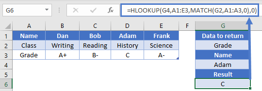

So, the MATCH function will evaluate to 3, and that tells the HLOOKUP to return a result from the 3^rd row in the A1:E3 range. Overall, we then get our desired result of “C”. Our formula is dynamic now in that we can change either the row to look at or the name to search for.

HLOOKUP limitations

As mentioned at the beginning of the article, the biggest downfall of HLOOKUP is that it requires the search term to be found in the left most column of the search range. While there are some fancy tricks you can do to overcome this (like the CHOOSE Function), the common alternative is to use INDEX and MATCH. That combo gives you more flexibility, and it can sometimes even be a faster calculation.

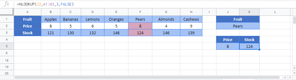
HLOOKUP in Google Sheets

The HLOOKUP Function works exactly the same in Google Sheets as in Excel:

 

HLOOKUP Examples in VBA

You can also use the HLOOKUP function in VBA. Type:

application.worksheetfunction.hlookup(lookup_value,table_array,row_index_num,range_lookup)

Executing the following VBA statements

Range("G2")=Application.WorksheetFunction.HLookup(Range("C1"),Range("A1:E3"),1)
Range("H2")=Application.WorksheetFunction.HLookup(Range("C1"),Range("A1:E3"),2)
Range("I2")=Application.WorksheetFunction.HLookup(Range("C1"),Range("A1:E3"),3)
Range("G3")=Application.WorksheetFunction.HLookup(Range("D1"),Range("A1:E3"),1)
Range("H3")=Application.WorksheetFunction.HLookup(Range("D1"),Range("A1:E3"),2)
Range("I3")=Application.WorksheetFunction.HLookup(Range("D1"),Range("A1:E3"),3)

will produce the following results

For the function arguments (lookup_value, etc.), you can either enter them directly into the function, or define variables to use instead.